前言
retinanet是我以前学了很久的目标检测框架,我将剖析下它的论文和代码。

论文地址
https://arxiv.org/abs/1708.02002
github地址
https://github.com/yanjingke/retinanet-keras
预备知识
1.tf.where()
定义如下:
where(condition, x=None, y=None,name=None)
condition:一个Tensor,数据类型为tf.bool类型
如果x、y均为空,那么返回condition中值为True的位置的Tensor:例如:x就是condition,y是返回值
如果x、y不为空,那么x、y必须有相同的形状。如果x、y是标量,那么condition参数也必须是标量。如果x、y是向量,那么condition必须和x的第一维有相同的形状或者和x形状一致。
返回值:如果x、y不为空的话,返回值和x、y有相同的形状,如果condition对应位置值为True那么返回Tensor对应位置
import tensorflow as tf
import numpy as np
sess=tf.Session()

#-------------------#
#   用法1:
#   x,y没值的时候
#-------------------#
a=[[[True, False], [True, False]], [[False, True], [False, True]], [[False, False], [False, True]]]
print(sess.run(tf.where(a)))
#-------------------#
#   用法2:
#   x,y有值的时候
#-------------------#
a=np.array([[1,0,0],[0,1,1]])
a1=np.array([[3,2,3],[4,5,6]])

print(sess.run(tf.equal(a,1)))
print(sess.run(tf.where(tf.equal(a,1),a,a1)))
- 1
- 2
- 3
- 4
- 5
- 6
- 7
- 8
- 9
- 10
- 11
- 12
- 13
- 14
- 15
- 16
- 17
- 18
- 19
- 20
- 21
- 22
- 23
- 24
[[0 0 0]
 [0 1 0]
 [1 0 1]
 [1 1 1]
 [2 1 1]]
[[ True False False]
 [False  True  True]]
[[1 2 3]
 [4 1 1]]
- 1
- 2
- 3
- 4
- 5
- 6
- 7
- 8
- 9
2. retinanet—anchor解读
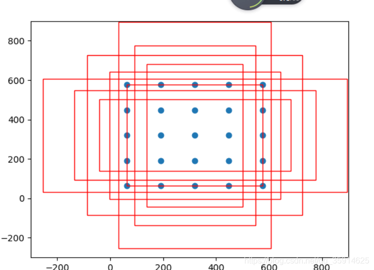
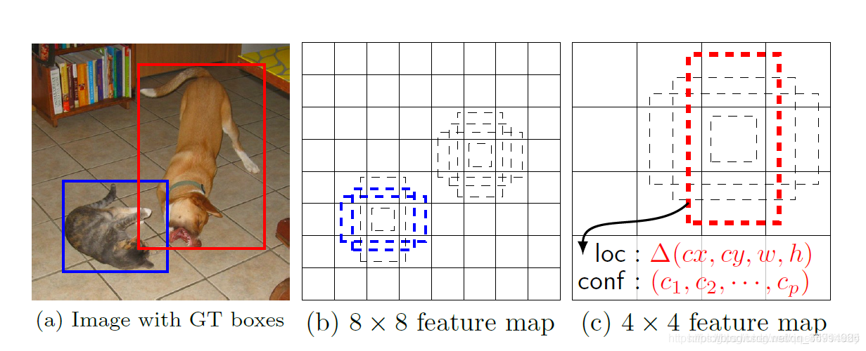
anchor的设置,相当于提前在图片上做预选,通常在生成anchor时,每一张图片上将会对应成千上万的anchor也就是候选框,可想而知,如此庞大的候选框数量,肯定能够满足对图上实例进行检测的需要,效果如下图所示

我计算了下retinanet的anchor数量大概有67995个。那么有了这些框框,网络便可以学习这些框框中的事物以及框框的位置,最终可以进行分类和回归
每个anchor-size对应着三种scale和三个ratio,那么每个anchor-size将对应生成9个先验框,同时生成的所有先验框均满足:
1.同一种scale,面积相同,形状不同
2.同一种ratio,形状相同,面积不同
3.对于scale和ratio的理解:scale指anchor的大小(可以当做宽)、ratio即为宽高比
anchor实现步骤:
1.因为我们最终的每个网格是是9个先验框,所以利用scale和ratio的长度相乘得到9
2.我们最终获得的anchor里面存放的是左上角和右下角的偏移量,最终生成(9x4)的数组
我以anchor大小为32的作为介绍。
sizes = [32, 64, 128, 256, 512],#anchor大小 strides = [8, 16, 32, 64, 128],#比例 ratios = np.array([0.5, 1, 2], keras.backend.floatx()), scales = np.array([2 ** 0, 2 ** (1.0 / 3.0), 2 ** (2.0 / 3.0)], keras.backend.floatx()), if ratios is None: ratios = AnchorParameters.default.ratios if scales is None: scales = AnchorParameters.default.scales num_anchors = len(ratios) * len(scales) anchors = np.zeros((num_anchors, 4))
- 1
- 2
- 3
- 4
- 5
- 6
- 7
- 8
- 9
- 10
- 11
- 12
- 13
- 14
首先生成[9,4]大小全为0的矩阵:
[[0. 0. 0. 0.] [0. 0. 0. 0.] [0. 0. 0. 0.] [0. 0. 0. 0.] [0. 0. 0. 0.] [0. 0. 0. 0.] [0. 0. 0. 0.] [0. 0. 0. 0.] [0. 0. 0. 0.]]
- 1
- 2
- 3
- 4
- 5
- 6
- 7
- 8
- 9
- 10
- 11
接下来,需要求解以w=h=32为基础的9种anchor的宽和高。
首先,我们需要求出三种scale的anchor对应的宽(W),此时只是做scale变换,不涉及ratios,自然所求的anchor都是大小不一的正方形。
 # 2.XY轴都复制,或只沿着Y轴复制的方法 # np.tile(a,(2,1))第一个参数为Y轴扩大倍数,第二个为X轴扩大倍数。本例中X轴扩大一倍便为不复制。
  anchors[:, 2:] = 32 * np.tile(scales, (2, len(ratios))).T
- 1
- 2
- 3
生成anchor_size=32在三种scale下的9个宽、高。第一列即为宽、第二列即为高。这样我们便得到了9个大小不一的正方形anchor。
[[32. 32. ] [40.317474 40.317474] [50.796833 50.796833] [32. 32. ] [40.317474 40.317474] [50.796833 50.796833] [32. 32. ] [40.317474 40.317474] [50.796833 50.796833]]
- 1
- 2
- 3
- 4
- 5
- 6
- 7
- 8
- 9
- 10
接下来将做ratio变换:
ratio变换的实质:将以上生成的正方形anchor按照一定比例缩放,求得缩放后的宽,保持scale不变,求得高。
求出每个anchor的面积,
然后求出每个anchor按照比例缩放后,得到的宽和高:
areas = anchors[:, 2] * anchors[:, 3]
anchors[:, 2] = np.sqrt(areas / np.repeat(ratios, len(scales)))
anchors[:, 3] = anchors[:, 2] * np.repeat(ratios, len(scales))
- 1
- 2
- 3
[[ 45.254834 22.627417 ] [ 57.01751905 28.50875952] [ 71.83757021 35.9187851 ] [ 32. 32. ] [ 40.31747437 40.31747437] [ 50.79683304 50.79683304] [ 22.627417 45.254834 ] [ 28.50875952 57.01751905] [ 35.9187851 71.83757021]]
- 1
- 2
- 3
- 4
- 5
- 6
- 7
- 8
- 9
然而我们anchor数组为
[[  0. 0. 45.254834 22.627417  ]
 [  0. 0. 57.01751905  28.50875952]
 [  0. 0. 71.83757021  35.9187851 ]
 [  0. 0. 32. 32. ]
 [  0. 0. 40.31747437  40.31747437]
 [  0. 0. 50.79683304  50.79683304]
 [  0. 0. 22.627417 45.254834  ]
 [  0. 0. 28.50875952  57.01751905]
 [  0. 0. 35.9187851   71.83757021]]
- 1
- 2
- 3
- 4
- 5
- 6
- 7
- 8
- 9
这种形式的坐标,并不是我们想要的,因为它只记录了当前anchor的宽和高。并没有给出坐标信息。
那么我们采取的办法是,以当前anchor的中心点为坐标原点建立直角坐标系,求出左上角坐标和右下角坐标,存入当前数组,格式为(x1,y1,x2,y2)。
anchors[:, 0::2] -= np.tile(anchors[:, 2] * 0.5, (2, 1)).T
anchors[:, 1::2] -= np.tile(anchors[:, 3] * 0.5, (2, 1)).T
- 1
- 2
此时的anchor数组为:
[[-22.627417   -11.3137085   22.627417 11.3137085 ]
 [-28.50875952 -14.25437976  28.50875952  14.25437976]
 [-35.9187851  -17.95939255  35.9187851   17.95939255]
 [-16. -16. 16. 16. ]
 [-20.15873718 -20.15873718  20.15873718  20.15873718]
 [-25.39841652 -25.39841652  25.39841652  25.39841652]
 [-11.3137085  -22.627417 11.3137085   22.627417  ]
 [-14.25437976 -28.50875952  14.25437976  28.50875952]
 [-17.95939255 -35.9187851   17.95939255  35.9187851 ]]
- 1
- 2
- 3
- 4
- 5
- 6
- 7
- 8
- 9
将anchor偏移量叠加到到原图上
以上我们得到的只是当前anchor相对于自身中心点的坐标,我们还要将anchor映射到特征金字塔的每一层的feature map上,我们以p3为例,p3的尺度为7575。
那么映射的思路为:
首先生成7575的网格坐标,对于每一个网格,将9个anchor分别嵌入进去,得到基于网格的anchor坐标。我们加了0.5,我们为什么要加0.5,其实我们把75*75看成网格,那么我们所求的网格点坐标其实都是每个小网格中心点的坐标,网格的边长是1。中心点肯定是要乘上0.5的。
shift_x = (np.arange(0, shape[1], dtype=keras.backend.floatx()) + 0.5) * stride shift_y = (np.arange(0, shape[0], dtype=keras.backend.floatx()) + 0.5) * stride shift_x, shift_y = np.meshgrid(shift_x, shift_y) shift_x = np.reshape(shift_x, [-1]) shift_y = np.reshape(shift_y, [-1]) shifts = np.stack([ shift_x, shift_y, shift_x, shift_y ], axis=0) shifts = np.transpose(shifts)
- 1
- 2
- 3
- 4
- 5
- 6
- 7
- 8
- 9
- 10
- 11
- 12
最终我们得到的结果为:
[[   4. 4. 4. 4.]
 [  12. 4.   12. 4.]
 [  20. 4.   20. 4.]
 ...,
 [ 580.  596.  580.  596.]
 [ 588.  596.  588.  596.]
 [ 596.  596.  596.  596.]]
- 1
- 2
- 3
- 4
- 5
- 6
- 7
此处我们构造了和anchor相同的结构,网格上第一列和第三列、第二列和第四列都是相同的。第一列是网格上75x75个点的横坐标,第二列是75x75个点的纵坐标。接下来,我们便可以直接做映射。
在上述中,我们得到的anchor坐标实际上可以看做是以anchor本身的中心点为坐标原点得到的,那么坐标值实际上可以看做是左上角和右下角两个点对中心点的偏移量。那么如果我们将中心点换做p3的feature map的网格点,然后将偏移量叠加至上面,不就完成了anchor到feature map的映射嘛。
代码:
number_of_anchors = np.shape(anchors)[0] k = np.shape(shifts)[0] shifted_anchors = np.reshape(anchors, [1, number_of_anchors, 4]) + np.array(np.reshape(shifts, [k, 1, 4]), keras.backend.floatx()) shifted_anchors = np.reshape(shifted_anchors, [k * number_of_anchors, 4])
- 1
- 2
- 3
- 4
得到的映射结果为:
[[ -18.627417 -7.3137085 26.627417 15.3137085 ]
 [ -24.50875952  -10.25437976   32.50875952   18.25437976]
 [ -31.9187851   -13.95939255   39.9187851 21.95939255]
 ...,
 [ 584.6862915   573.372583 607.3137085   618.627417  ]
 [ 581.74562024  567.49124048  610.25437976  624.50875952]
 [ 578.04060745  560.0812149   613.95939255  631.9187851 ]]
- 1
- 2
- 3
- 4
- 5
- 6
- 7
具体代码对应我github上Vision_For_prior.py文件。
3.retinanet—focalloss解读
Focal loss是针对这种情况重新设计的CE loss来解决类别不平衡问题.
在one-stage的网络中,假设正负样本的比例达到1:10000,就会出现两个问题,一是样本不平衡,二是负样本主导loss,虽然负样本的loss小,但是由于大量的负样本是easy example,大量负样本是准确率很高的第0类,但是数量很多加起来loss甚至大于正样本的loss;在one-stage的网络中loss由负样本主导,但是负样本大多数准确率很高,经过focal loss后变成了正负样本共同主导.
总结
1、控制正负样本的权重
2、控制容易分类和难分类样本的权重
正负样本:
一张图像可能生成成千上万的候选框,但是其中只有很少一部分是包含目标的的,有目标的就是正样本,没有目标的就是负样本。
容易分类和难分类样本:
假设存在一个二分类,样本1预测概率为0.9,样本2预测概率0.3,显然前者更可能是样本1,其就是容易分类的样本;后者有可能是其他类别,所以其为难分类样本。
正负样本控制
在focalloss了解focalloss时候我们来介绍下什么是交叉熵损失函数:
y=1为正样本,otherwise为负样本

这里用pt代替p和(1-p)化简上式:

想要降低负样本的影响,可以在常规的损失函数前增加一个系数αt。与Pt类似,当label=1的时候,αt=α;当label=otherwise的时候,αt=1 - α,a的范围也是0到1。此时我们便可以通过设置α实现控制正负样本对loss的贡献。
其中:


控制容易分类和难分类样本的权重
假设存在一个二分类,样本1预测概率为0.9,样本2预测概率0.3,显然前者更可能是样本1,其就是容易分类的样本;后者有可能是其他类别,所以其为难分类样本。
论文中实现方式为:

其中下面为称为调制系数(modulating factor)

总结:
1、当pt趋于0的时候,调制系数趋于1,对于总的loss的贡献很大。当pt趋于1的时候,调制系数趋于0,也就是对于总的loss的贡献很小。
2、当γ=0的时候,focal loss就是传统的交叉熵损失,可以通过调整γ实现调制系数的改变。
通过如下公式就可以实现控制正负样本的权重和控制容易分类和难分类样本的权重。

代码:
def focal(alpha=0.25, gamma=2.0): def _focal(y_true, y_pred): # y_true [batch_size, num_anchor, num_classes+1] # y_pred [batch_size, num_anchor, num_classes] labels = y_true[:, :, :-1] anchor_state = y_true[:, :, -1] # -1 是需要忽略的, 0 是背景, 1 是存在目标 classification = y_pred # 找出存在目标的先验框 indices_for_object = backend.where(keras.backend.equal(anchor_state, 1)) labels_for_object = backend.gather_nd(labels, indices_for_object) classification_for_object = backend.gather_nd(classification, indices_for_object) # 计算每一个先验框应该有的权重 alpha_factor_for_object = keras.backend.ones_like(labels_for_object) * alpha alpha_factor_for_object = backend.where(keras.backend.equal(labels_for_object, 1), alpha_factor_for_object, 1 - alpha_factor_for_object) # aa = K.print_tensor(labels_for_object, message='y_true = ') focal_weight_for_object = backend.where(keras.backend.equal(labels_for_object, 1), 1 - classification_for_object, classification_for_object) focal_weight_for_object = alpha_factor_for_object * focal_weight_for_object ** gamma # 将权重乘上所求得的交叉熵 cls_loss_for_object = focal_weight_for_object * keras.backend.binary_crossentropy(labels_for_object, classification_for_object) # 找出实际上为背景的先验框 indices_for_back = backend.where(keras.backend.equal(anchor_state, 0)) labels_for_back = backend.gather_nd(labels, indices_for_back) classification_for_back = backend.gather_nd(classification, indices_for_back) # 计算每一个先验框应该有的权重 alpha_factor_for_back = keras.backend.ones_like(labels_for_back) * (1 - alpha) focal_weight_for_back = classification_for_back focal_weight_for_back = alpha_factor_for_back * focal_weight_for_back ** gamma # 将权重乘上所求得的交叉熵 cls_loss_for_back = focal_weight_for_back * keras.backend.binary_crossentropy(labels_for_back, classification_for_back) # 标准化,实际上是正样本的数量 normalizer = tf.where(keras.backend.equal(anchor_state, 1)) normalizer = keras.backend.cast(keras.backend.shape(normalizer)[0], keras.backend.floatx()) normalizer = keras.backend.maximum(keras.backend.cast_to_floatx(1.0), normalizer) # 将所获得的loss除上正样本的数量 cls_loss_for_object = keras.backend.sum(cls_loss_for_object) cls_loss_for_back = keras.backend.sum(cls_loss_for_back) # 总的loss loss = (cls_loss_for_object + cls_loss_for_back)/normalizer return loss return _focal
- 1
- 2
- 3
- 4
- 5
- 6
- 7
- 8
- 9
- 10
- 11
- 12
- 13
- 14
- 15
- 16
- 17
- 18
- 19
- 20
- 21
- 22
- 23
- 24
- 25
- 26
- 27
- 28
- 29
- 30
- 31
- 32
- 33
- 34
- 35
- 36
- 37
- 38
- 39
- 40
- 41
- 42
- 43
- 44
- 45
- 46
- 47
- 48
- 49
- 50
- 51
retinanet 代码讲解
1.预测部分
主干特征提取resnet50
采用Inverted residual在3x3网络结构前利用1x1卷积降维,在3x3网络结构后,利用1x1卷积升维,相比直接使用3x3网络卷积效果更好,参数更少,先进行压缩,再进行扩张。
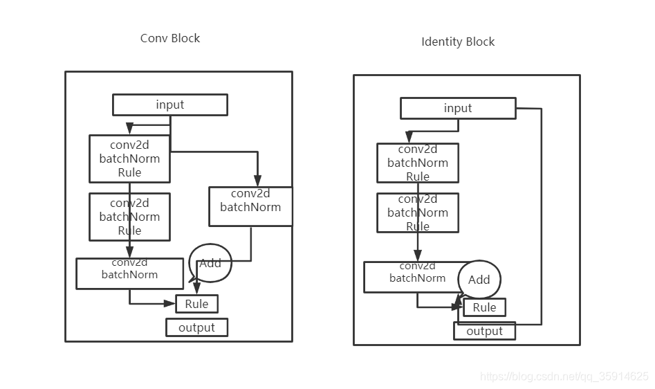
在Resnet50中他有两个结构分别名为Conv Block和Identity Block,Conv block输入和输出是是不同的,而Identity Block输入和输出是相同的。这样做意味着后面的特征层的内容会有一部分由其前面的某一层线性贡献。
总的resnet50结构

我们取出长宽压缩了三次、四次、五次的结果来进行特征提取
#-------------------------------------------------------------#
#   ResNet50的网络部分
#-------------------------------------------------------------#
from __future__ import print_function

import numpy as np
from keras import layers

from keras.layers import Input
from keras.layers import Dense,Conv2D,MaxPooling2D,ZeroPadding2D,AveragePooling2D
from keras.layers import Activation,BatchNormalization,Flatten
from keras.models import Model

from keras.preprocessing import image
import keras.backend as K
from keras.utils.data_utils import get_file
from keras.applications.imagenet_utils import decode_predictions
from keras.applications.imagenet_utils import preprocess_input


def identity_block(input_tensor, kernel_size, filters, stage, block): filters1, filters2, filters3 = filters conv_name_base = 'res' + str(stage) + block + '_branch' bn_name_base = 'bn' + str(stage) + block + '_branch' x = Conv2D(filters1, (1, 1), name=conv_name_base + '2a',use_bias=False)(input_tensor) x = BatchNormalization(name=bn_name_base + '2a')(x) x = Activation('relu')(x) x = Conv2D(filters2, kernel_size,padding='same', name=conv_name_base + '2b',use_bias=False)(x) x = BatchNormalization(name=bn_name_base + '2b')(x) x = Activation('relu')(x) x = Conv2D(filters3, (1, 1), name=conv_name_base + '2c',use_bias=False)(x) x = BatchNormalization(name=bn_name_base + '2c')(x) x = layers.add([x, input_tensor]) x = Activation('relu')(x) return x


def conv_block(input_tensor, kernel_size, filters, stage, block, strides=(2, 2)): filters1, filters2, filters3 = filters conv_name_base = 'res' + str(stage) + block + '_branch' bn_name_base = 'bn' + str(stage) + block + '_branch' x = Conv2D(filters1, (1, 1), strides=strides, name=conv_name_base + '2a',use_bias=False)(input_tensor) x = BatchNormalization(name=bn_name_base + '2a')(x) x = Activation('relu')(x) x = Conv2D(filters2, kernel_size, padding='same', name=conv_name_base + '2b',use_bias=False)(x) x = BatchNormalization(name=bn_name_base + '2b')(x) x = Activation('relu')(x) x = Conv2D(filters3, (1, 1), name=conv_name_base + '2c',use_bias=False)(x) x = BatchNormalization(name=bn_name_base + '2c')(x) shortcut = Conv2D(filters3, (1, 1), strides=strides, name=conv_name_base + '1',use_bias=False)(input_tensor) shortcut = BatchNormalization(name=bn_name_base + '1')(shortcut) x = layers.add([x, shortcut]) x = Activation('relu')(x) return x


def ResNet50(inputs): img_input = inputs x = ZeroPadding2D((3, 3))(img_input) # 300,300,64 x = Conv2D(64, (7, 7), strides=(2, 2), name='conv1',use_bias=False)(x) x = BatchNormalization(name='bn_conv1')(x) x = Activation('relu')(x) # 150,150,64 x = MaxPooling2D((3, 3), strides=(2, 2), padding="same")(x) # 150,150,256 x = conv_block(x, 3, [64, 64, 256], stage=2, block='a', strides=(1, 1)) x = identity_block(x, 3, [64, 64, 256], stage=2, block='b') x = identity_block(x, 3, [64, 64, 256], stage=2, block='c') y0 = x # 75,75,512 x = conv_block(x, 3, [128, 128, 512], stage=3, block='a') x = identity_block(x, 3, [128, 128, 512], stage=3, block='b') x = identity_block(x, 3, [128, 128, 512], stage=3, block='c') x = identity_block(x, 3, [128, 128, 512], stage=3, block='d') y1 = x # 38,38,1024 x = conv_block(x, 3, [256, 256, 1024], stage=4, block='a') x = identity_block(x, 3, [256, 256, 1024], stage=4, block='b') x = identity_block(x, 3, [256, 256, 1024], stage=4, block='c') x = identity_block(x, 3, [256, 256, 1024], stage=4, block='d') x = identity_block(x, 3, [256, 256, 1024], stage=4, block='e') x = identity_block(x, 3, [256, 256, 1024], stage=4, block='f') y2 = x # 19,19,2048 x = conv_block(x, 3, [512, 512, 2048], stage=5, block='a') x = identity_block(x, 3, [512, 512, 2048], stage=5, block='b') x = identity_block(x, 3, [512, 512, 2048], stage=5, block='c') y3 = x model = Model(img_input, [y0,y1,y2,y3], name='resnet50') return model

if __name__ == "__main__": inputs = Input(shape=(600, 600, 3)) model = ResNet50(inputs) model.summary()
- 1
- 2
- 3
- 4
- 5
- 6
- 7
- 8
- 9
- 10
- 11
- 12
- 13
- 14
- 15
- 16
- 17
- 18
- 19
- 20
- 21
- 22
- 23
- 24
- 25
- 26
- 27
- 28
- 29
- 30
- 31
- 32
- 33
- 34
- 35
- 36
- 37
- 38
- 39
- 40
- 41
- 42
- 43
- 44
- 45
- 46
- 47
- 48
- 49
- 50
- 51
- 52
- 53
- 54
- 55
- 56
- 57
- 58
- 59
- 60
- 61
- 62
- 63
- 64
- 65
- 66
- 67
- 68
- 69
- 70
- 71
- 72
- 73
- 74
- 75
- 76
- 77
- 78
- 79
- 80
- 81
- 82
- 83
- 84
- 85
- 86
- 87
- 88
- 89
- 90
- 91
- 92
- 93
- 94
- 95
- 96
- 97
- 98
- 99
- 100
- 101
- 102
- 103
- 104
- 105
- 106
- 107
- 108
- 109
- 110
- 111
- 112
- 113
- 114
特征金字塔构建,获得预测结果
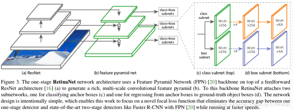
通过前面的特征提取我们获得五个特征层,分别是P3、P4、P5、P6、P7。他们的大小分别是(75x75x256)(38x38x256)(19x19x256)(10x10x256)(5x5x256)
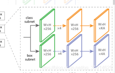
获得的所有特征层经过同一个class subnet和同一个box subnet 获得了预测结果
class subnet采用4次256通道的卷积和1次num_priors x num_classes的卷积,num_priors为anchor的数量,num_classes为种类,这里我们采用的是voc数据集所以种类为20。
box subnet采用4次256通道的卷积和1次num_priors x 4的卷积,num_priors指的是该特征层所拥有的先验框数量,4指的是先验框的调整情况。
def make_last_layer_loc(num_classes,num_anchors,pyramid_feature_size=256): inputs = keras.layers.Input(shape=(None, None, pyramid_feature_size)) options = { 'kernel_size' : 3, 'strides' : 1, 'padding' : 'same', 'kernel_initializer' : keras.initializers.normal(mean=0.0, stddev=0.01, seed=None), 'bias_initializer'   : 'zeros' } outputs = inputs for i in range(4): outputs = keras.layers.Conv2D(filters=256,activation='relu',name='pyramid_regression_{}'.format(i),**options)(outputs) outputs = keras.layers.Conv2D(num_anchors * 4, name='pyramid_regression', **options)(outputs) regression = keras.layers.Reshape((-1, 4), name='pyramid_regression_reshape')(outputs) regression_model = keras.models.Model(inputs=inputs, outputs=regression, name="regression_submodel") return regression_model


def make_last_layer_cls(num_classes,num_anchors,pyramid_feature_size=256): inputs = keras.layers.Input(shape=(None, None, pyramid_feature_size)) options = { 'kernel_size' : 3, 'strides' : 1, 'padding' : 'same', } classification = [] outputs = inputs for i in range(4): outputs = keras.layers.Conv2D( filters=256, activation='relu', name='pyramid_classification_{}'.format(i), kernel_initializer=keras.initializers.normal(mean=0.0, stddev=0.01, seed=None), bias_initializer='zeros', **options )(outputs) outputs = keras.layers.Conv2D(filters=num_classes * num_anchors, kernel_initializer=keras.initializers.normal(mean=0.0, stddev=0.01, seed=None), bias_initializer=PriorProbability(probability=0.01), name='pyramid_classification'.format(), **options )(outputs) outputs = keras.layers.Reshape((-1, num_classes), name='pyramid_classification_reshape')(outputs) classification = keras.layers.Activation('sigmoid', name='pyramid_classification_sigmoid')(outputs) classification_model = keras.models.Model(inputs=inputs, outputs=classification, name="classification_submodel") return classification_model


def resnet_retinanet(num_classes, inputs=None, num_anchors=None, submodels=None, name='retinanet'): if inputs==None: inputs = keras.layers.Input(shape=(600, 600, 3)) else: inputs = inputs resnet = ResNet50(inputs) if num_anchors is None: num_anchors = AnchorParameters.default.num_anchors() C3, C4, C5 = resnet.outputs[1:] P5 = keras.layers.Conv2D(256, kernel_size=1, strides=1, padding='same', name='C5_reduced')(C5) # 38x38x256 P5_upsampled = layers.UpsampleLike(name='P5_upsampled')([P5, C4]) P5 = keras.layers.Conv2D(256, kernel_size=3, strides=1, padding='same', name='P5')(P5) # 38x38x256 P4 = keras.layers.Conv2D(256, kernel_size=1, strides=1, padding='same', name='C4_reduced')(C4) P4 = keras.layers.Add(name='P4_merged')([P5_upsampled, P4]) P4_upsampled = layers.UpsampleLike(name='P4_upsampled')([P4, C3]) P4 = keras.layers.Conv2D(256, kernel_size=3, strides=1, padding='same', name='P4')(P4) # 75x75x256 P3 = keras.layers.Conv2D(256, kernel_size=1, strides=1, padding='same', name='C3_reduced')(C3) P3 = keras.layers.Add(name='P3_merged')([P4_upsampled, P3]) P3 = keras.layers.Conv2D(256, kernel_size=3, strides=1, padding='same', name='P3')(P3) P6 = keras.layers.Conv2D(256, kernel_size=3, strides=2, padding='same', name='P6')(C5) P7 = keras.layers.Activation('relu', name='C6_relu')(P6) P7 = keras.layers.Conv2D(256, kernel_size=3, strides=2, padding='same', name='P7')(P7) features =  [P3, P4, P5, P6, P7] regression_model = make_last_layer_loc(num_classes,num_anchors) classification_model = make_last_layer_cls(num_classes,num_anchors) regressions = [] classifications = [] for feature in features: regression = regression_model(feature) classification = classification_model(feature) regressions.append(regression) classifications.append(classification) regressions = keras.layers.Concatenate(axis=1, name="regression")(regressions) classifications = keras.layers.Concatenate(axis=1, name="classification")(classifications) pyramids = [regressions,classifications] model = keras.models.Model(inputs=inputs, outputs=pyramids, name=name) return model
- 1
- 2
- 3
- 4
- 5
- 6
- 7
- 8
- 9
- 10
- 11
- 12
- 13
- 14
- 15
- 16
- 17
- 18
- 19
- 20
- 21
- 22
- 23
- 24
- 25
- 26
- 27
- 28
- 29
- 30
- 31
- 32
- 33
- 34
- 35
- 36
- 37
- 38
- 39
- 40
- 41
- 42
- 43
- 44
- 45
- 46
- 47
- 48
- 49
- 50
- 51
- 52
- 53
- 54
- 55
- 56
- 57
- 58
- 59
- 60
- 61
- 62
- 63
- 64
- 65
- 66
- 67
- 68
- 69
- 70
- 71
- 72
- 73
- 74
- 75
- 76
- 77
- 78
- 79
- 80
- 81
- 82
- 83
- 84
- 85
- 86
- 87
- 88
- 89
- 90
- 91
- 92
- 93
- 94
- 95
- 96
- 97
- 98
- 99
- 100
- 101
- 102
- 103
- 104
- 105
- 106
- 107
- 108
- 109
- 110
- 111
- 112
- 113
- 114
- 115
- 116
预测结果的解码
预测框的解码部分,我们通过主干网络和特征金字塔获得了
num_priors x 4的卷积 用于预测 该特征层上 每一个网格点上 每一个先验框的变化情况。
num_priors x num_classes的卷积 用于预测 该特征层上 每一个网格点上 每一个预测框对应的种类。
利用预设好的 预先设定好的9个anchor框进行调整。
先验框虽然可以代表一定的框的位置信息与框的大小信息,但是其是有限的,无法表示任意情况,因此还需要调整,Retinanet利用4次256通道的卷积+num_priors x 4的卷积的结果对先验框进行调整。
num_priors x 4中的num_priors表示了这个网格点所包含的先验框数量,其中的4表示了框的左上角xy轴,右下角xy的调整情况。
def decode_boxes(self, mbox_loc, mbox_priorbox): # 获得先验框的宽与高 prior_width = mbox_priorbox[:, 2] - mbox_priorbox[:, 0] prior_height = mbox_priorbox[:, 3] - mbox_priorbox[:, 1] # 获取真实框的左上角与右下角 decode_bbox_xmin = mbox_loc[:,0]*prior_width*0.2 + mbox_priorbox[:, 0] decode_bbox_ymin = mbox_loc[:,1]*prior_height*0.2 + mbox_priorbox[:, 1] decode_bbox_xmax = mbox_loc[:,2]*prior_width*0.2 + mbox_priorbox[:, 2] decode_bbox_ymax = mbox_loc[:,3]*prior_height*0.2 + mbox_priorbox[:, 3] # 真实框的左上角与右下角进行堆叠 decode_bbox = np.concatenate((decode_bbox_xmin[:, None], decode_bbox_ymin[:, None], decode_bbox_xmax[:, None], decode_bbox_ymax[:, None]), axis=-1) # 防止超出0与1 decode_bbox = np.minimum(np.maximum(decode_bbox, 0.0), 1.0) return decode_bbox
- 1
- 2
- 3
- 4
- 5
- 6
- 7
- 8
- 9
- 10
- 11
- 12
- 13
- 14
- 15
- 16
- 17
- 18
- 19
当然得到最终的获得真实框的调整结果后,取出取出每一类得分大于confidence_threshold的框和得分。利用框的位置和得分进行非极大抑制,得到最终结果。
非极大抑制的执行过程如下所示:
1、对所有图片进行循环。
2、找出该图片中得分大于门限函数的框。在进行重合框筛选前就进行得分的筛选可以大幅度减少框的数量。
3、判断第2步中获得的框的种类与得分。取出预测结果中框的位置与之进行堆叠。此时最后一维度里面的内容由5+num_classes变成了4+1+2,四个参数代表框的位置,一个参数代表预测框是否包含物体,两个参数分别代表种类的置信度与种类。
4、对种类进行循环,非极大抑制的作用是筛选出一定区域内属于同一种类得分最大的框,对种类进行循环可以帮助我们对每一个类分别进行非极大抑制。
5、根据得分对该种类进行从大到小排序。
6、每次取出得分最大的框,计算其与其它所有预测框的重合程度,重合程度过大的则剔除。
 def detection_out(self, predictions, mbox_priorbox, background_label_id=0, keep_top_k=200, confidence_threshold=0.4): # 网络预测的结果 mbox_loc = predictions[0] # 置信度 mbox_conf = predictions[1] # 先验框 mbox_priorbox = mbox_priorbox results = [] # 对每一个图片进行处理 for i in range(len(mbox_loc)): decode_bbox = self.decode_boxes(mbox_loc[i], mbox_priorbox) bs_class_conf = mbox_conf[i] class_conf = np.expand_dims(np.max(bs_class_conf, 1),-1) class_pred = np.expand_dims(np.argmax(bs_class_conf, 1),-1) conf_mask = (class_conf >= confidence_threshold)[:,0] detections = np.concatenate((decode_bbox[conf_mask], class_conf[conf_mask], class_pred[conf_mask]), 1) unique_class = np.unique(detections[:,-1]) best_box = [] if len(unique_class) == 0: results.append(best_box) continue # 对种类进行循环, # 非极大抑制的作用是筛选出一定区域内属于同一种类得分最大的框, # 对种类进行循环可以帮助我们对每一个类分别进行非极大抑制。 for c in unique_class: cls_mask = detections[:,-1] == c detection = detections[cls_mask] scores = detection[:,4] # 根据得分对该种类进行从大到小排序。 arg_sort = np.argsort(scores)[::-1] detection = detection[arg_sort] while np.shape(detection)[0]>0: # 每次取出得分最大的框,计算其与其它所有预测框的重合程度,重合程度过大的则剔除。 best_box.append(detection[0]) if len(detection) == 1: break ious = iou(best_box[-1],detection[1:]) detection = detection[1:][ious<self._nms_thresh] results.append(best_box) # 获得,在所有预测结果里面,置信度比较高的框 # 还有,利用先验框和retinanet的预测结果,处理获得了真实框(预测框)的位置 return results

def iou(b1,b2): b1_x1, b1_y1, b1_x2, b1_y2 = b1[0], b1[1], b1[2], b1[3] b2_x1, b2_y1, b2_x2, b2_y2 = b2[:, 0], b2[:, 1], b2[:, 2], b2[:, 3] inter_rect_x1 = np.maximum(b1_x1, b2_x1) inter_rect_y1 = np.maximum(b1_y1, b2_y1) inter_rect_x2 = np.minimum(b1_x2, b2_x2) inter_rect_y2 = np.minimum(b1_y2, b2_y2) inter_area = np.maximum(inter_rect_x2 - inter_rect_x1, 0) * \ np.maximum(inter_rect_y2 - inter_rect_y1, 0) area_b1 = (b1_x2-b1_x1)*(b1_y2-b1_y1) area_b2 = (b2_x2-b2_x1)*(b2_y2-b2_y1) iou = inter_area/np.maximum((area_b1+area_b2-inter_area),1e-6) return iou
- 1
- 2
- 3
- 4
- 5
- 6
- 7
- 8
- 9
- 10
- 11
- 12
- 13
- 14
- 15
- 16
- 17
- 18
- 19
- 20
- 21
- 22
- 23
- 24
- 25
- 26
- 27
- 28
- 29
- 30
- 31
- 32
- 33
- 34
- 35
- 36
- 37
- 38
- 39
- 40
- 41
- 42
- 43
- 44
- 45
- 46
- 47
- 48
- 49
- 50
- 51
- 52
- 53
- 54
- 55
- 56
- 57
- 58
- 59
- 60
- 61
- 62
- 63
- 64
- 65
- 66
- 67
- 68
- 69
- 70
2.训练部分
真实框的编码
在我们出入网络的时候真实框并不是和预测值相同类型数值,所以不能直接训练和计算loss。**我们需要转换成对于Retinanet网络的预测结果的的格式信息。**从预测结果获得真实框的过程被称作解码,而从真实框获得预测结果的过程就是编码的过程。
def encode_box(self, box, return_iou=True): iou = self.iou(box) encoded_box = np.zeros((self.num_priors, 4 + return_iou)) # 找到每一个真实框,重合程度较高的先验框 assign_mask = iou > self.overlap_threshold if not assign_mask.any(): assign_mask[iou.argmax()] = True if return_iou: encoded_box[:, -1][assign_mask] = iou[assign_mask] # 找到对应的先验框 assigned_priors = self.priors[assign_mask] # 逆向编码,将真实框转化为Retinanet预测结果的格式 assigned_priors_w = (assigned_priors[:, 2] - assigned_priors[:, 0]) assigned_priors_h = (assigned_priors[:, 3] - assigned_priors[:, 1]) encoded_box[:,0][assign_mask] = (box[0] - assigned_priors[:, 0])/assigned_priors_w/0.2 encoded_box[:,1][assign_mask] = (box[1] - assigned_priors[:, 1])/assigned_priors_h/0.2 encoded_box[:,2][assign_mask] = (box[2] - assigned_priors[:, 2])/assigned_priors_w/0.2 encoded_box[:,3][assign_mask] = (box[3] - assigned_priors[:, 3])/assigned_priors_h/0.2 return encoded_box.ravel()
- 1
- 2
- 3
- 4
- 5
- 6
- 7
- 8
- 9
- 10
- 11
- 12
- 13
- 14
- 15
- 16
- 17
- 18
- 19
- 20
- 21
- 22
- 23
- 24
- 25
- 26
但是由于原始图片中可能存在多个真实框,可能同一个先验框会与多个真实框重合度较高,我们只取其中与真实框重合度最高的就可以了。
我们还要经过一次筛选,iou最大的那个真实框筛选出来。
我们会忽略一些重合度相对较高但是不是非常高的先验框,一般将重合度在0.4-0.5之间的先验框进行忽略。
def ignore_box(self, box): iou = self.iou(box) ignored_box = np.zeros((self.num_priors, 1)) # 找到每一个真实框,重合程度较高的先验框 assign_mask = (iou > self.ignore_threshold)&(iou<self.overlap_threshold) if not assign_mask.any(): assign_mask[iou.argmax()] = True ignored_box[:, 0][assign_mask] = iou[assign_mask] return ignored_box.ravel() def assign_boxes(self, boxes): assignment = np.zeros((self.num_priors, 4 + 1 + self.num_classes + 1)) assignment[:, 4] = 0.0 assignment[:, -1] = 0.0 if len(boxes) == 0: return assignment # 对每一个真实框都进行iou计算 # print(boxes[:, :4].shape) ingored_boxes = np.apply_along_axis(self.ignore_box, 1, boxes[:, :4]) # print(ingored_boxes.shape ) # 取重合程度最大的先验框,并且获取这个先验框的index ingored_boxes = ingored_boxes.reshape(-1, self.num_priors, 1) # (num_priors) ignore_iou = ingored_boxes[:, :, 0].max(axis=0) # (num_priors) ignore_iou_mask = ignore_iou > 0 assignment[:, 4][ignore_iou_mask] = -1 assignment[:, -1][ignore_iou_mask] = -1 # (n, num_priors, 5) encoded_boxes = np.apply_along_axis(self.encode_box, 1, boxes[:, :4]) # 每一个真实框的编码后的值,和iou # (n, num_priors) encoded_boxes = encoded_boxes.reshape(-1, self.num_priors, 5) # 取重合程度最大的先验框,并且获取这个先验框的index # (num_priors) best_iou = encoded_boxes[:, :, -1].max(axis=0) # (num_priors) best_iou_idx = encoded_boxes[:, :, -1].argmax(axis=0) # (num_priors) best_iou_mask = best_iou > 0 # 某个先验框它属于哪个真实框 best_iou_idx = best_iou_idx[best_iou_mask] assign_num = len(best_iou_idx) # 保留重合程度最大的先验框的应该有的预测结果 # 哪些先验框存在真实框 encoded_boxes = encoded_boxes[:, best_iou_mask, :] assignment[:, :4][best_iou_mask] = encoded_boxes[best_iou_idx,np.arange(assign_num),:4] # 4代表为背景的概率,为0 assignment[:, 4][best_iou_mask] = 1 assignment[:, 5:-1][best_iou_mask] = boxes[best_iou_idx, 4:] assignment[:, -1][best_iou_mask] = 1 # 通过assign_boxes我们就获得了,输入进来的这张图片,应该有的预测结果是什么样子的 return assignment
- 1
- 2
- 3
- 4
- 5
- 6
- 7
- 8
- 9
- 10
- 11
- 12
- 13
- 14
- 15
- 16
- 17
- 18
- 19
- 20
- 21
- 22
- 23
- 24
- 25
- 26
- 27
- 28
- 29
- 30
- 31
- 32
- 33
- 34
- 35
- 36
- 37
- 38
- 39
- 40
- 41
- 42
- 43
- 44
- 45
- 46
- 47
- 48
- 49
- 50
- 51
- 52
- 53
- 54
- 55
- 56
- 57
- 58
- 59
- 60
- 61
- 62
- 63
- 64
loss值计算
最后我们将进行focalloss和smoothloos。focalloss进行交叉熵计算,smoothloss就行回归计算
focalloss我就不多做介绍了,smooth有空讲吧
def rand(a=0, b=1): return np.random.rand()*(b-a) + a

def focal(alpha=0.25, gamma=2.0): def _focal(y_true, y_pred): # y_true [batch_size, num_anchor, num_classes+1] # y_pred [batch_size, num_anchor, num_classes] labels = y_true[:, :, :-1] anchor_state   = y_true[:, :, -1]  # -1 是需要忽略的, 0 是背景, 1 是存在目标 classification = y_pred # 找出存在目标的先验框 indices_for_object = backend.where(keras.backend.equal(anchor_state, 1)) labels_for_object = backend.gather_nd(labels, indices_for_object) classification_for_object = backend.gather_nd(classification, indices_for_object) # 计算每一个先验框应该有的权重 alpha_factor_for_object = keras.backend.ones_like(labels_for_object) * alpha alpha_factor_for_object = backend.where(keras.backend.equal(labels_for_object, 1), alpha_factor_for_object, 1 - alpha_factor_for_object) # aa = K.print_tensor(labels_for_object, message='y_true = ') focal_weight_for_object = backend.where(keras.backend.equal(labels_for_object, 1), 1 - classification_for_object, classification_for_object) focal_weight_for_object = alpha_factor_for_object * focal_weight_for_object ** gamma # 将权重乘上所求得的交叉熵 cls_loss_for_object = focal_weight_for_object * keras.backend.binary_crossentropy(labels_for_object, classification_for_object) # 找出实际上为背景的先验框 indices_for_back = backend.where(keras.backend.equal(anchor_state, 0)) labels_for_back = backend.gather_nd(labels, indices_for_back) classification_for_back = backend.gather_nd(classification, indices_for_back) # 计算每一个先验框应该有的权重 alpha_factor_for_back = keras.backend.ones_like(labels_for_back) * (1 - alpha) focal_weight_for_back = classification_for_back focal_weight_for_back = alpha_factor_for_back * focal_weight_for_back ** gamma # 将权重乘上所求得的交叉熵 cls_loss_for_back = focal_weight_for_back * keras.backend.binary_crossentropy(labels_for_back, classification_for_back) # 标准化,实际上是正样本的数量 normalizer = tf.where(keras.backend.equal(anchor_state, 1)) normalizer = keras.backend.cast(keras.backend.shape(normalizer)[0], keras.backend.floatx()) normalizer = keras.backend.maximum(keras.backend.cast_to_floatx(1.0), normalizer) # 将所获得的loss除上正样本的数量 cls_loss_for_object = keras.backend.sum(cls_loss_for_object) cls_loss_for_back = keras.backend.sum(cls_loss_for_back) # 总的loss loss = (cls_loss_for_object + cls_loss_for_back)/normalizer return loss return _focal

def smooth_l1(sigma=3.0): sigma_squared = sigma ** 2 def _smooth_l1(y_true, y_pred): # y_true [batch_size, num_anchor, 4+1] # y_pred [batch_size, num_anchor, 4] regression = y_pred regression_target = y_true[:, :, :-1] anchor_state = y_true[:, :, -1] # 找到正样本 indices = tf.where(keras.backend.equal(anchor_state, 1)) regression = tf.gather_nd(regression, indices) regression_target = tf.gather_nd(regression_target, indices) # 计算 smooth L1 loss # f(x) = 0.5 * (sigma * x)^2 if |x| < 1 / sigma / sigma # |x| - 0.5 / sigma / sigma otherwise regression_diff = regression - regression_target regression_diff = keras.backend.abs(regression_diff) regression_loss = backend.where( keras.backend.less(regression_diff, 1.0 / sigma_squared), 0.5 * sigma_squared * keras.backend.pow(regression_diff, 2), regression_diff - 0.5 / sigma_squared ) normalizer = keras.backend.maximum(1, keras.backend.shape(indices)[0]) normalizer = keras.backend.cast(normalizer, dtype=keras.backend.floatx()) loss = keras.backend.sum(regression_loss) / normalizer return loss return _smooth_l1
- 1
- 2
- 3
- 4
- 5
- 6
- 7
- 8
- 9
- 10
- 11
- 12
- 13
- 14
- 15
- 16
- 17
- 18
- 19
- 20
- 21
- 22
- 23
- 24
- 25
- 26
- 27
- 28
- 29
- 30
- 31
- 32
- 33
- 34
- 35
- 36
- 37
- 38
- 39
- 40
- 41
- 42
- 43
- 44
- 45
- 46
- 47
- 48
- 49
- 50
- 51
- 52
- 53
- 54
- 55
- 56
- 57
- 58
- 59
- 60
- 61
- 62
- 63
- 64
- 65
- 66
- 67
- 68
- 69
- 70
- 71
- 72
- 73
- 74
- 75
- 76
- 77
- 78
- 79
- 80
- 81
- 82
- 83
- 84
- 85
- 86
- 87
文章来源: blog.csdn.net,作者:快了的程序猿小可哥,版权归原作者所有,如需转载,请联系作者。
原文链接:blog.csdn.net/qq_35914625/article/details/108357512